
Multi-beam LiDAR
MotrixSim 0.10.0 introduces multi-beam LiDAR based on physical collision geometry. The sensor outputs point clouds in the world coordinate frame for robot obstacle avoidance, terrain perception, localization and mapping, and reinforcement-learning observations. Real-time point-cloud visualization helps verify the mounting pose and scan results.
Run from the motrixsim-docs directory:
uv run examples/control/robot_locomotion.py --robot go2 --scene playground --lidar ouster_os1_rev6_32ch_10hz_512res
MJCF Configuration
LiDAR configuration in MJCF consists of three parts: body/site defines the mounting position and orientation, asset/lidar defines a reusable model and scan geometry, and sensor/lidar attaches the sensor to a specified site.
<asset>
  <lidar name="grid_64" cutoff="25" pattern="grid"
         hscan="1024" vscan="64" hrange="-180 180" vrange="-15 15"/>
</asset>
<worldbody>
  <body name="robot">
    <site name="lidar_site" pos="0.25 0 0.20" quat="0.5 0.5 0.5 0.5"/>
  </body>
</worldbody>
<sensor>
  <lidar name="roof_lidar" asset="grid_64" site="lidar_site"
         exclude="parentsubtree"/>
</sensor>| site.pos / site.quat | Set the LiDAR mounting position and orientation on the robot. |
| asset/lidar.name | Define a reusable LiDAR profile name for sensor instances. |
| cutoff | Set the maximum ray distance in metres. |
| pattern | Select the scan pattern: grid for a uniform grid or rings for a rotating multi-line scan. |
| hscan / vscan | Set the horizontal and vertical samples per frame, which determine Grid point-cloud resolution. |
| hrange / vrange | Set horizontal and vertical scan-angle ranges in degrees. |
| sensor/lidar.asset | Reference the LiDAR profile defined under asset. |
| sensor/lidar.site | Specify the mounting site that defines ray origins and directions. |
| exclude | Configure filtering for the robot's own colliders; parentsubtree can be used for multi-link robots. |
| hz | Optional full-scan frequency; when omitted, a complete scan is generated at every simulation step. |
Reading Sensor Data
After each step(), read the point cloud with get_sensor_value(). The example below reshapes a Grid point cloud to (1024, 64, 3); missed rays are represented by zero vectors:
model.step(data)
points = model.get_sensor_value("roof_lidar", data).reshape(1024, 64, 3)
hit_points = points[(points != 0).any(axis=-1)]
Performance
The results below come from an end-to-end Python benchmark in the playground scene. Each LiDAR uses a 1024×64 Grid with hz omitted, producing 65,536 rays per simulation step. Tests ran on an AMD Ryzen 9 9950X (16 cores, 32 threads), with the median of three rounds reported. Measurements cover the full physics pipeline within model.step() and exclude rendering.
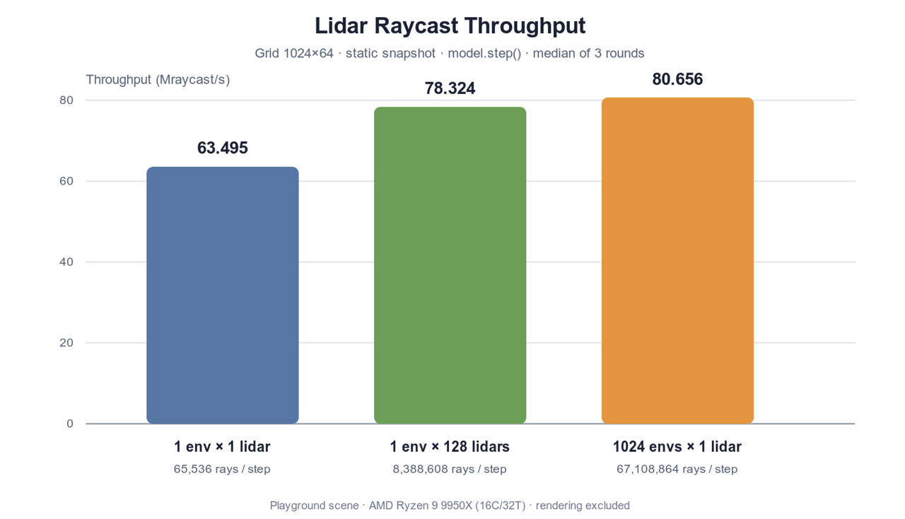
With one LiDAR in each of 1,024 parallel environments, aggregate throughput reached approximately 80.656 million raycasts per second. This is a measured result for the software and hardware configuration described above, not the peak throughput of an isolated raycast kernel.
cd motrixsim-python/motrixsim-docs
uv run python examples/bench/lidar.py --case all